Anna Liski

Straightening Algorithm for Profilometry Data Correction

Python

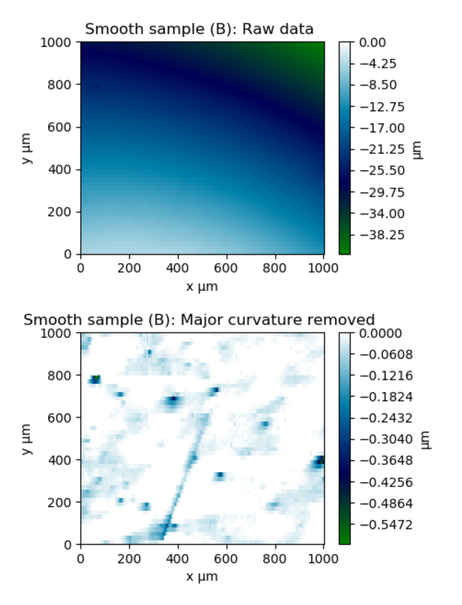
Data: Surface topography of a metal sample measured by stylus profilometry.

Objective: Study the depth of pores in the alloy’s microstructure. Profilometry resolution was sufficient, but tilt and polishing-induced curvature obscured the pores.

Method: A straightening algorithm was applied to the profilometry data. Polynomial functions of progressively increasing degree were fitted to the raw data, and the resulting fits were subtracted iteratively. This procedure corrected surface tilt and removed major curvature, allowing the true surface profile to emerge.

Outcome: The surface roughness originating from the alloy’s porous microstructure became clearly visible, providing a more accurate representation of the sample’s true topography.

Simple UI for Convolution

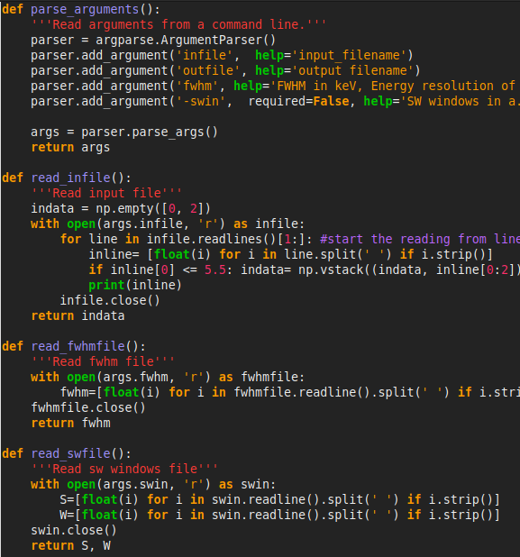
Python, Shell Script

Data: Computational momentum distribution data.

Objective: Convolution codes were obtained from a collaborator. They were well-written, but difficult to apply without knowledge of Python.

Method: I created a simple text-based UI in Python that uses the convolution codes as modules. This enabled one-line execution from the Linux terminal with user-specified parameters and file I/O.

Outcome: Made the advanced Python scripts written by the collaborator easily usable by all lab members.

Arrhenius Law Fit for Hydrogen Absorption

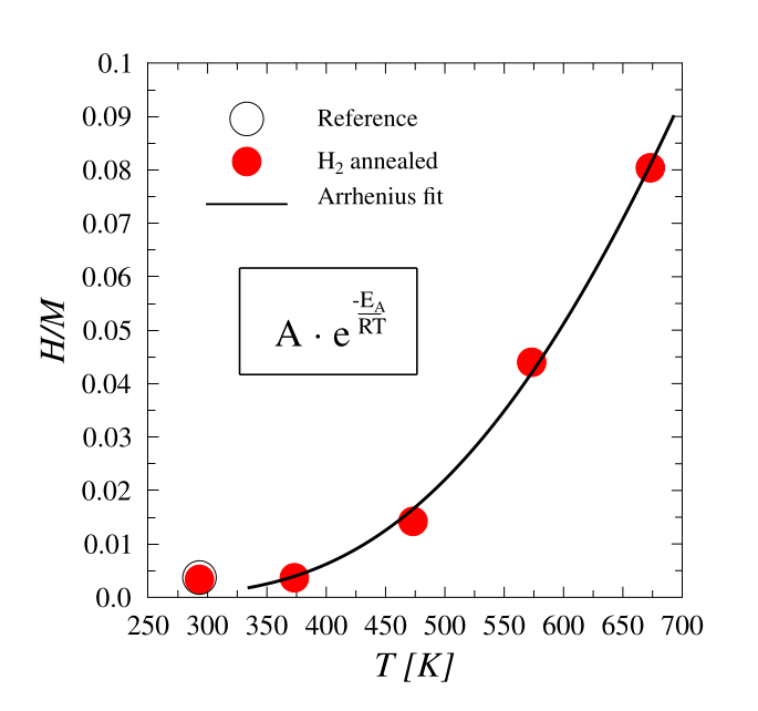
Python

Data: Ion beam analysis of hydrogen concentration in a metal.

Objective: Determine the hydrogen absorption activation energy.

Method: The activation energy was obtained by fitting the Arrhenius model to the experimental data. Samples were saturated with hydrogen at different temperatures for the experiments.

Outcome: The Arrhenius fit yielded an activation energy of E_A = 0.22 ± 0.02 eV, with goodness of fit R² = 0.997.

Elemental Composition Visualization

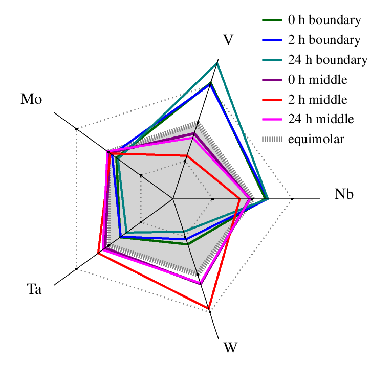
Python, Graphics Layout Engine

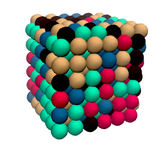
Data: Energy Dispersive X-ray measurements of an advanced metal alloy.

Objective: Study the elemental composition of a five-element metal alloy (V, Mo, Ta, W, Nb) and create an intuitive visualization comparing grain center, grain boundary, and the ideal alloy.

Method: Using Python for statistical analysis of Energy Dispersive X-ray data and a graphics layout engine, I created a five-axis spider plot. Colors highlighted grain centers (red–purple) and boundaries (green–blue), while the ideal equimolar composition was shown as a dashed line with shaded regions indicating deviations.

Outcome: The visualization makes it clear at a glance how elemental composition differs between measured regions and how each compares to the ideal alloy.

Statistical Analysis Fitting

Python

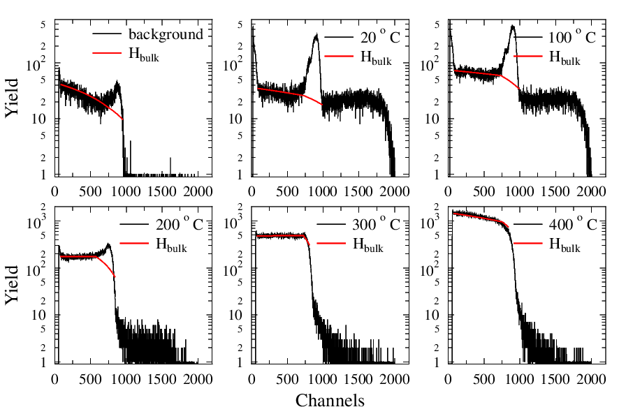
Data: Statistical data from Elastic Recoil Detection Analysis (ERDA).

Objective: Quantify the amount of hydrogen residing in the bulk of the metal sample.

Method: The raw ERDA signal includes both surface hydrogen and hydrogen absorbed into the metal. The analysis removes the surface hydrogen contribution by fitting the bulk signal shape, isolating the absorbed hydrogen signal. This allows the study of hydrogen absorption at different temperatures.

Outcome: The total absorbed hydrogen content was successfully calculated using this approach.

Monte Carlo Simulation of Hydrogen Diffusion

Python, Fortran (pre-written)

Simulation: Modeling 3D diffusion of a single hydrogen atom in a metal lattice.

Objective: Investigate hydrogen trapping in metal defects and determine the sink strength for different defect types.

Method: Hydrogen diffusion is simulated atom by atom using a 3D random walk until the atom is trapped. Different defect types and concentrations are considered, and sink strength is calculated from the number of steps before trapping.

Outcome: Sink strength parameters were determined for spherical traps, dislocations, and grain boundary defects, providing insight into defect-related hydrogen behavior in metals.

First-Principles Modeling

Python, VASP + CSC, VESTA

Simulation: Metal structures are built with Python and relaxed on a supercomputer using VASP. The models include BCC metal alloys, vacancies, and, in some cases, hydrogen interactions with vacancies and metal atoms. The simulation relaxes the structure to its minimal energy, revealing naturally occurring behavior and enabling calculation of energies associated with hydrogen interactions.

Outcome: Provided atomistic-level understanding of hydrogen interaction with metals and defects, offering a solid theoretical explanation for macroscopic observations.

Stopping and Range of Ions in Matter

SRIM

Simulation: SRIM is a simulation software used to model the interaction of ions with matter. It calculates ion penetration depth, energy deposition, and defect creation in materials, allowing the prediction of material modifications from ion irradiation.

Outcome: SRIM is used to plan and optimize ion beam experiments. By simulating ion ranges and interaction profiles in advance, it enables experiment design, anticipates material responses, and minimizes trial-and-error in the lab.

Sample Stage Automation

LabVIEW

Objective: Automate the measurement of numerous tree rings, which is impractical manually, by developing a remote-controlled sample holder for precise X-Y positioning during ion beam analysis.

Method: LabVIEW was used to control two stepper motors for X and Y movement. The graphical user interface allows manual positioning as well as uploading coordinate files for automated measurements. The sample stage is connected to the measurement system, enabling automatic movement and synchronized measurement, creating a fully automated workflow.

Outcome: An automated X-Y sample stage capable of running pre-programmed measurement sequences independently.

Fossil Database Statistical Evaluation

Python

Database: NOW (New and Old Worlds) mammal fossil database.

Objective: Study patterns of mammalian speciation over time.

Method: The dataset was cleaned and processed considering localities and sampling. Logistic regression curves were fitted to estimate the significance of occurrences, and geographic maps were created to visualize fossil distributions globally.

Outcome: Identified statistically significant patterns of speciation and provided a clear global visualization of fossil mammal distributions over time and space.

Analysis of Insect Observation Data

Python

Database: NINA (Norwegian Institute for Nature Research) insect observation database.

Objective: Analyze the database to identify the most common insect species observed in Norway over time.

Method: Processed and cleaned the dataset, then generated histogram visualizations to study species frequency and yearly observation trends.

Outcome: Identified the most frequently observed insect species in Norway and revealed temporal patterns in species observations over the years.